Graph-based Random Walk

This notebook is used to construct a Human-Mouse graph through Random Walk method.

Introduction

Human diffusion-based tractography

• We utilized diffusion data from the Human Connectome Project (HCP), which have been preprocessed following HCP’s standard pipeline.

• Further post-processing steps of tractography were carried out using MRtrix3.

Mouse Tracer

• Tracer data maps neural connectivity by tracking the movement of injected tracers along axonal pathways in animal brains.

• The mouse connectome data we used was initially sourced from the Allen Mouse Connectivity Atlas.

Embedding space generated from Human-Mouse graph

• Intra-species edges are defined by anatomical connectivity, derived from mouse viral tracer data and human tractography.

• Cross-species edges were established using transcriptomic latent embeddings from DNN model, constrained by coarse-scale anatomical hierarchies.

• For the pruned Human-Mouse graph, we used the Node2vec algorithm by Sporns et al. to construct graph embedding.

Define human and mouse ROIs

%matplotlib inline

human_select_cortex_region = ['A8m', 'A8dl', 'A9l', 'A6dl','A6m','A9m', 'A10m', 'A9/46d','IFJ', 'A46', 'A9/46v', 'A8vl','A6vl','A10l', 'A44d', 'IFS', 'A45c', 'A45r', 'A44op','A44v', 'A14m', 'A12/47o', 'A11l','A11m', 'A13', 'A12/47l','A32p','A32sg','A24cd','A24rv','A4hf', 'A6cdl', 'A4ul', 'A4t', 'A4tl', 'A6cvl','A1/2/3ll', 'A4ll','A1/2/3ulhf', 'A1/2/3tonIa', 'A2','A1/2/3tru','A7r', 'A7c', 'A5l', 'A7pc', 'A7ip', 'A39c', 'A39rd', 'A40rd', 'A40c', 'A39rv','A40rv',
                             'A7m', 'A5m', 'dmPOS','A31','A23d','A23c','A23v','cLinG', 'rCunG','cCunG', 'rLinG', 'vmPOS', 'mOccG', 'V5/MT+', 'OPC', 'iOccG', 'msOccG', 'lsOccG',
                             'G', 'vIa', 'dIa', 'vId/vIg', 'dIg', 'dId','A38m', 'A41/42', 'TE1.0 and TE1.2', 'A22c', 'A38l', 'A22r', 'A21c', 'A21r', 'A37dl', 'aSTS', 'A20iv', 'A37elv', 'A20r', 'A20il', 'A37vl', 'A20cl','A20cv', 'A20rv', 'A37mv', 'A37lv', 'A35/36r', 'A35/36c', 'lateral PPHC', 'A28/34', 'TH','TI','rpSTS','cpSTS']
mouse_select_cortex_region = ['ACAd', 'ACAv', 'PL','ILA', 'ORBl', 'ORBm', 'ORBvl','MOp','SSp-n', 'SSp-bfd', 'SSp-ll', 'SSp-m',
       'SSp-ul', 'SSp-tr', 'SSp-un','SSs','PTLp','RSPagl','RSPd', 'RSPv','VISpm','VISp','VISal','VISl','VISpl','AId','AIp','AIv','GU','VISC','TEa', 'PERI', 'ECT','AUDd', 'AUDp',
       'AUDpo', 'AUDv']

len(human_select_cortex_region)

105

len(mouse_select_cortex_region)

37

human_select_subcortex_region = ['mAmyg', 'lAmyg', 'CA1', 'CA4DG', 'CA2CA3', 'subiculum','Claustrum', 'head of caudate', 'body of caudate', 'Putamen',
       'posterovemtral putamen', 'nucleus accumbens','external segment of globus pallidus','internal segment of globus pallidus', 'mPMtha', 'Stha','cTtha', 'Otha',
        'mPFtha','lPFtha','rTtha', 'PPtha']
mouse_select_subcortex_region = ['LA', 'BLA', 'BMA', 'PA','CA1', 'CA2', 'CA3', 'DG', 'SUB', 'ACB', 'CP', 'FS', 'SF', 'SH','sAMY', 'PAL', 'VENT', 'SPF', 'SPA', 'PP', 'GENd', 'LAT', 'ATN',
       'MED', 'MTN', 'ILM', 'GENv', 'EPI', 'RT']

len(human_select_cortex_region+human_select_subcortex_region)

127

Human_select_region = human_select_cortex_region + human_select_subcortex_region
Mouse_select_region = mouse_select_cortex_region + mouse_select_subcortex_region

len(Human_select_region)

127

len(Mouse_select_region)

66

import warnings
warnings.filterwarnings('ignore')
import os
import pandas as pd
import numpy as np
import seaborn as sns
from matplotlib import pyplot as plt
import pickle

Load human structural connectivity data and region info table

Human_dti_dataframe=pd.read_csv('../../tutorials/structural_connection/human_127atlas_dti.csv')

Human_dti_dataframe.set_index('Unnamed: 0',drop=True,inplace=True)

human_127atlas = pd.read_excel('../../transbrain/atlas/roi_of_bn_atlas.xlsx')

human_127atlas

	Anatomical Name	Full Name	Atlas Type	Left Index	Right Index	Atlas Index
0	A8m	A8m, medial area 8	BN	1	2	1
1	A8dl	A8dl, dorsolateral area 8	BN	3	4	2
2	A9l	A9l, lateral area 9	BN	5	6	3
3	A6dl	A6dl, dorsolateral area 6	BN	7	8	4
4	A6m	A6m, medial area 6	BN	9	10	5
...	...	...	...	...	...	...
122	rTtha	rTtha, rostral temporal thalamus	BN	237	238	123
123	PPtha	PPtha, posterior parietal thalamus	BN	239	240	124
124	Otha	Otha, occipital thalamus	BN	241	242	125
125	cTtha	cTtha, caudal temporal thalamus	BN	243	244	126
126	lPFtha	lPFtha, lateral pre-frontal thalamus	BN	245	246	127

127 rows × 6 columns

Human_dti_dataframe.index = human_127atlas['Anatomical Name'].values.tolist()
Human_dti_dataframe.columns = human_127atlas['Anatomical Name'].values.tolist()

Human_dti_dataframe = Human_dti_dataframe[Human_select_region]
Human_dti_dataframe = Human_dti_dataframe.T[Human_select_region]

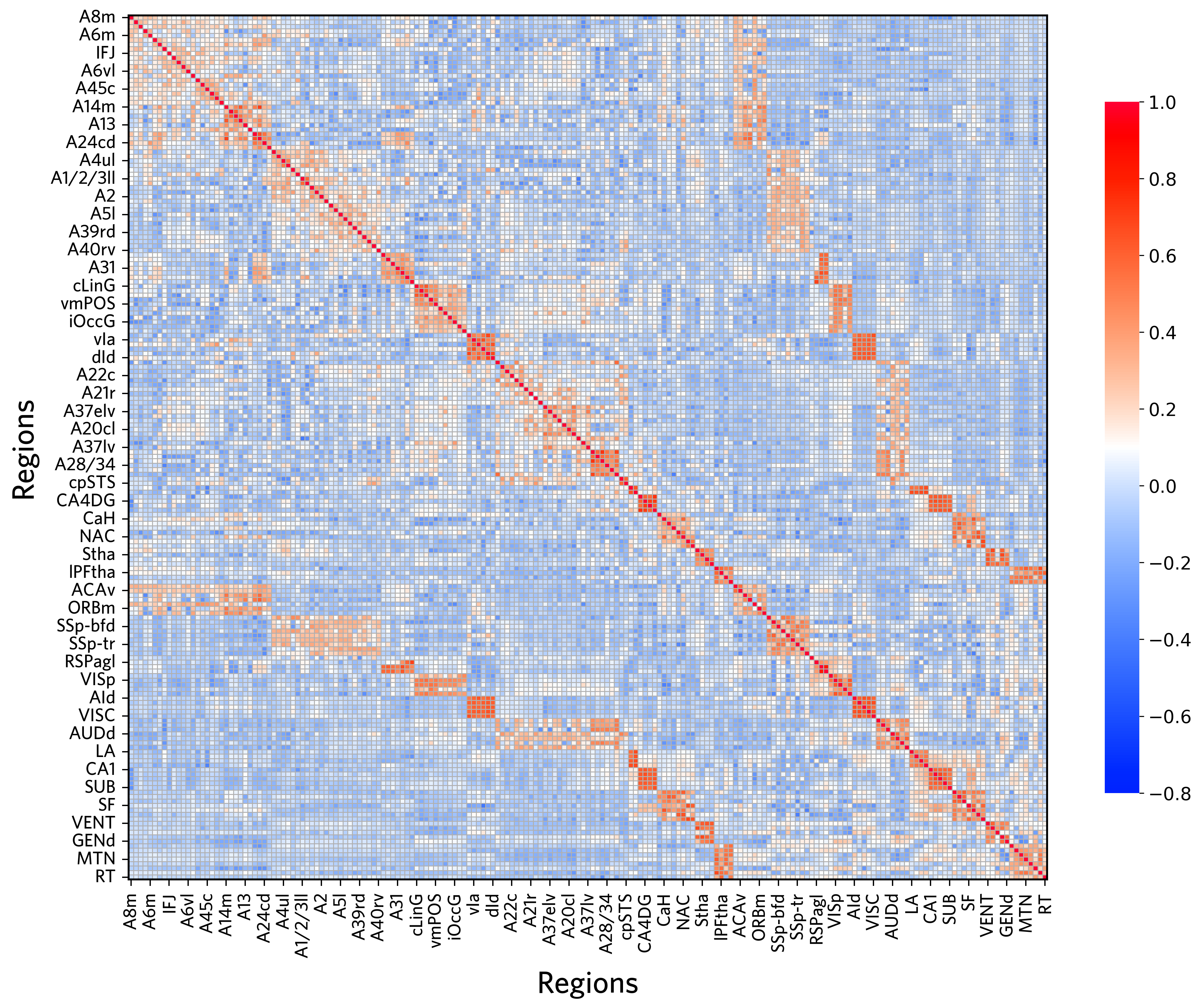
Visualize the structural connectivity matrix

f, ax = plt.subplots(figsize=(11, 9),dpi=600)
sns.heatmap(Human_dti_dataframe,linewidths=0.3,cmap='RdBu_r',vmin=0)
ax.set(xlabel="", ylabel="")

[Text(0.5, 421.3333333333332, ''), Text(652.3333333333331, 0.5, '')]

Load mouse tracer data

Mouse_tracer_dataframe = pd.read_csv('../../tutorials/structural_connection/mouse_atlas_tracer.csv')

Mouse_tracer_dataframe.set_index('Unnamed: 0',drop=True,inplace=True)

Mouse_tracer_dataframe = Mouse_tracer_dataframe[Mouse_select_region]
Mouse_tracer_dataframe = Mouse_tracer_dataframe.T[Mouse_select_region]

Visualize the mouse tracer matrix

f, ax = plt.subplots(figsize=(11, 9),dpi=600)
sns.heatmap(Mouse_tracer_dataframe,linewidths=0.3,cmap='RdBu_r',vmin=0)

<Axes: xlabel='Unnamed: 0'>

Load anatomical hierachy constraint information

hier_table = pd.read_excel('./files/hierarchical_brain_relationships.xlsx')

cortex_similarity_dataframe = pd.read_csv('./files/net_emd_mean_dataframe_cortex.csv') # Region-specific TR similarity from embeddings of detached model
cortex_similarity_dataframe.set_index('Unnamed: 0',inplace=True,drop=True)
cortex_similarity_dataframe = cortex_similarity_dataframe[human_select_cortex_region]
cortex_similarity_dataframe = cortex_similarity_dataframe.T[mouse_select_cortex_region].T

subcortex_similarity_dataframe = pd.read_csv('./files/net_emd_mean_dataframe_subcortex.csv')
subcortex_similarity_dataframe.set_index('Unnamed: 0',inplace=True,drop=True)
subcortex_similarity_dataframe = subcortex_similarity_dataframe.T[mouse_select_subcortex_region].T

corr_matrix_mean = np.zeros((len(Human_select_region),len(Mouse_select_region)))
corr_matrix_mean[:len(human_select_cortex_region),:len(mouse_select_cortex_region)] = cortex_similarity_dataframe.T.values
corr_matrix_mean[len(human_select_cortex_region):,len(mouse_select_cortex_region):] = subcortex_similarity_dataframe.T.values
corr_matrix_mean_dataframe = pd.DataFrame(corr_matrix_mean,index=Human_select_region,columns=Mouse_select_region)

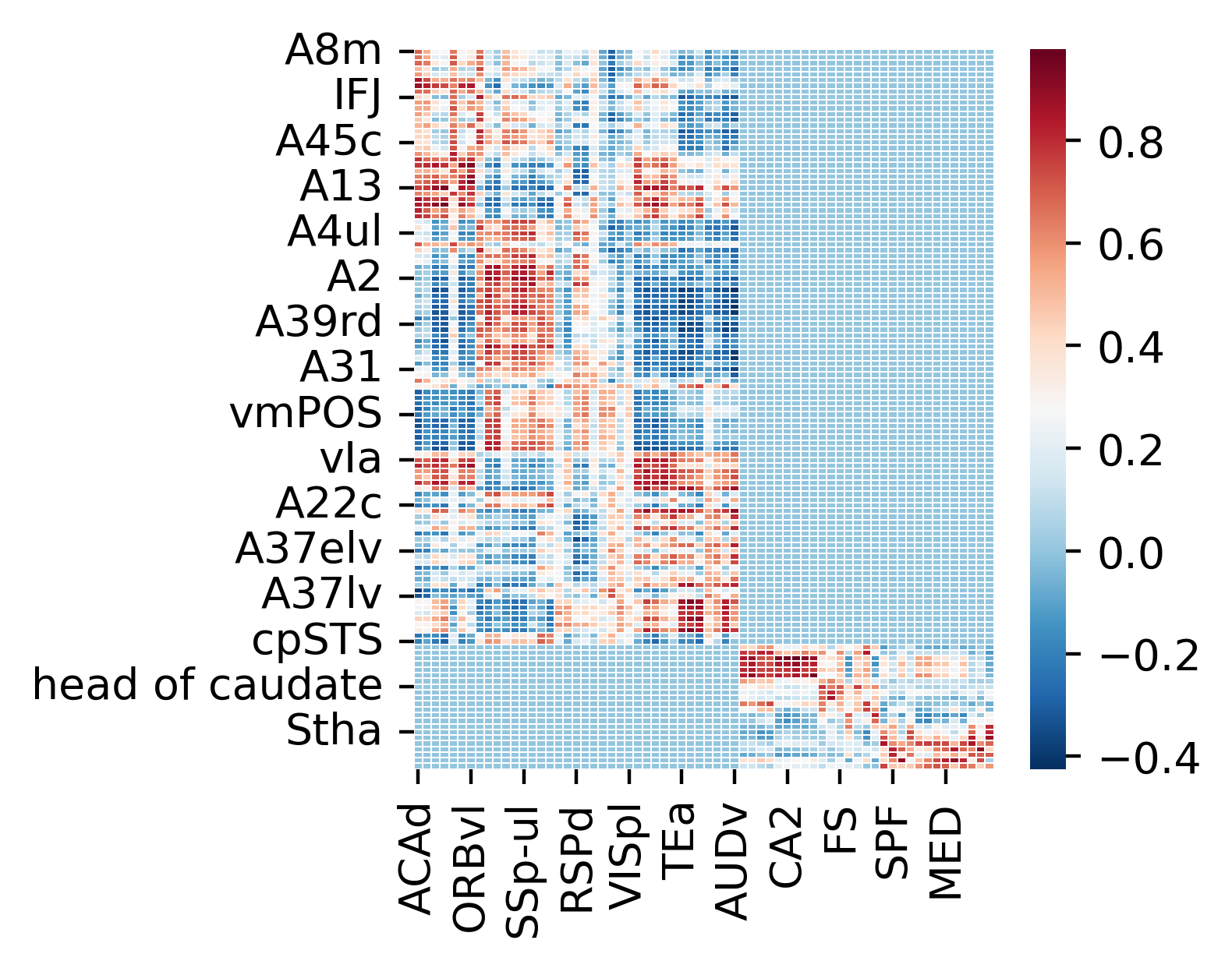
Visualization of cross-species transcriptional similarity with hierarchical constraints

fig,ax=plt.subplots(1,1,figsize=(3,3),dpi=400)
sns.heatmap(corr_matrix_mean_dataframe,cmap='RdBu_r',linewidths=0.3)
ax.set(xlabel="", ylabel="")

[Text(0.5, 16.888888888888864, ''), Text(34.888888888888864, 0.5, '')]

Sparse_matrix = np.zeros_like(corr_matrix_mean_dataframe.values)

Sparse_matrix_dataframe=pd.DataFrame(Sparse_matrix)

Sparse_matrix_dataframe.index = corr_matrix_mean_dataframe.index
Sparse_matrix_dataframe.columns = corr_matrix_mean_dataframe.columns

for i in range(11):
    for h_n in [item.strip().strip("'") for item in hier_table['Human Regions'].iloc[i].split(",")]:
        for m_n in [item.strip().strip("'") for item in hier_table['Mouse Regions'].iloc[i].split(",")]:
            Sparse_matrix_dataframe.loc[h_n,m_n] = corr_matrix_mean_dataframe.loc[h_n,m_n]

Sparse_matrix[Sparse_matrix<0]=0

fig,ax=plt.subplots(1,1,figsize=(3,3),dpi=400)
sns.heatmap(Sparse_matrix_dataframe,cmap='RdBu_r',linewidths=0.3,vmin=0)
ax.set(xlabel="", ylabel="")

[Text(0.5, 16.888888888888864, ''), Text(34.888888888888864, 0.5, '')]

embedding_input=np.zeros((193,193))
embedding_input[:127,:127] = Human_dti_dataframe.values
embedding_input[:127,127:] = Sparse_matrix_dataframe.values
embedding_input[127:,:127] = Sparse_matrix_dataframe.T.values
embedding_input[127:,127:] = Mouse_tracer_dataframe.values

region_labels = human_select_cortex_region + ['mAmyg', 'lAmyg', 'CA1', 'CA4DG', 'CA2CA3', 'subiculum', 'Claustrum','CaH','CaB', 'Putamen','PVP','NAC',
       'GPe','GPi', 'mPMtha','Stha', 'cTtha', 'Otha','mPFtha', 'lPFtha', 'rTtha', 'PPtha'] + Mouse_select_region

'mPMtha', 'Stha','cTtha', 'Otha',
        'mPFtha','lPFtha','rTtha', 'PPtha']

embedding_input = pd.DataFrame(embedding_input,index=region_labels,columns=region_labels)

from matplotlib import pyplot as plt
import seaborn as sns
from matplotlib.colors import LinearSegmentedColormap,Normalize
import matplotlib.colors as mcolors
import matplotlib
from matplotlib.font_manager import FontProperties
matplotlib.rcParams['axes.spines.right'] = False
matplotlib.rcParams['axes.spines.top'] = False
font_path ='../../tutorials/whitney-medium.otf'
custom_font = FontProperties(fname=font_path)
from matplotlib.patches import Rectangle

from matplotlib import pyplot as plt
import matplotlib.colors as mcolors
from matplotlib.colors import LinearSegmentedColormap,Normalize
from matplotlib.colors import LinearSegmentedColormap, rgb_to_hsv, hsv_to_rgb

original_cmap = plt.get_cmap("coolwarm")

colors = original_cmap(np.linspace(0, 1, 256))

def adjust_color(color, factor):

    r, g, b, a = color
    hsv = rgb_to_hsv([r, g, b])
    hsv[1] = min(1, hsv[1] * factor)
    hsv[2] = min(1, hsv[2] * factor)
    adjusted_rgb = hsv_to_rgb(hsv)
    return np.array([adjusted_rgb[0], adjusted_rgb[1], adjusted_rgb[2], a])

red_adjustment = 1.5
blue_adjustment = 1.5


for i in range(len(colors)):

    if colors[i, 2] > 0.5:
        colors[i] = adjust_color(colors[i], blue_adjustment)

    elif colors[i, 0] > 0.5:
        colors[i] = adjust_color(colors[i], red_adjustment)

custom_cmap = LinearSegmentedColormap.from_list("custom_coolwarm_adjusted", colors)

def brighten_cmap(cmap, factor=1.2):

    new_colors = []
    for c in cmap(np.linspace(0, 1, cmap.N)):
        new_color = mcolors.rgb_to_hsv(c[:3])
        new_color[2] = min(new_color[2] * factor, 1.0)
        new_colors.append(mcolors.hsv_to_rgb(new_color))
    return LinearSegmentedColormap.from_list("bright_plasma", new_colors)

bright_cmap = brighten_cmap(custom_cmap, factor=6)

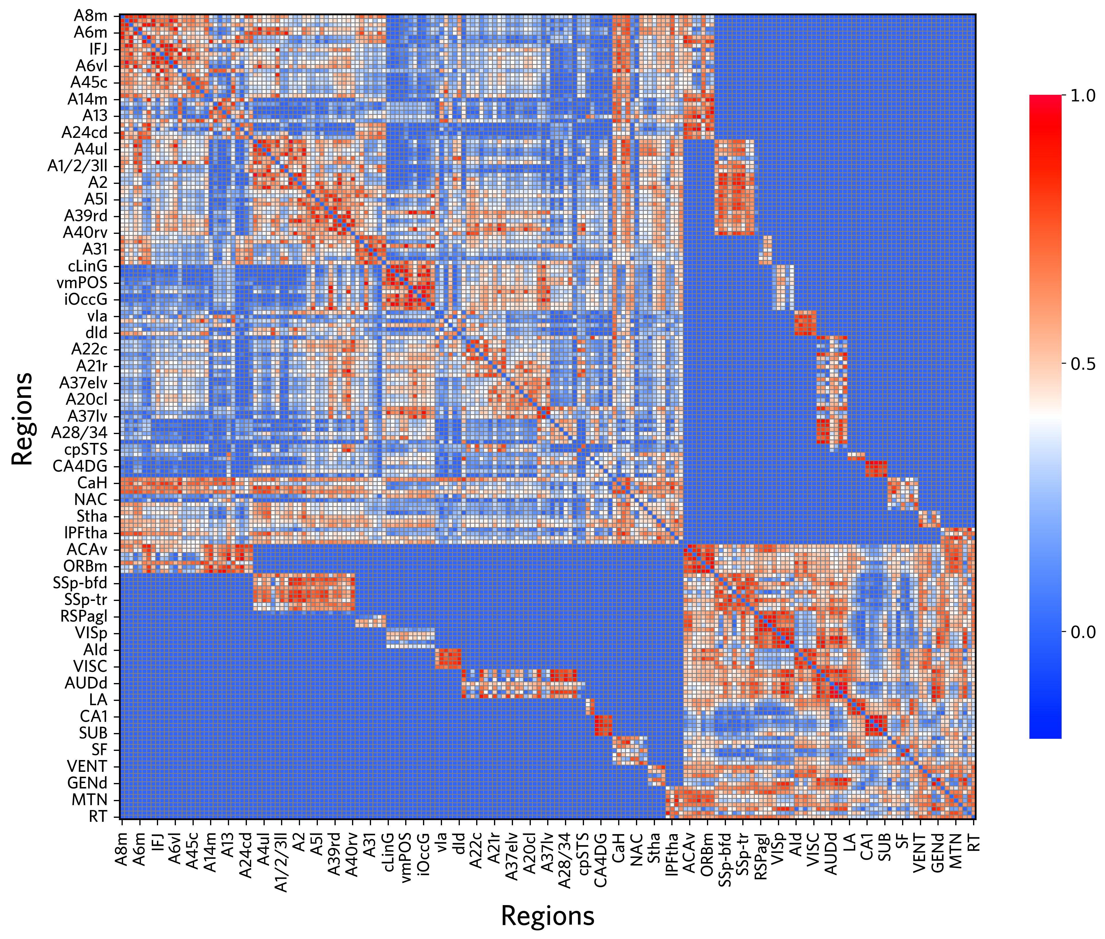
Visualization of the initial cross-species graph

f, ax = plt.subplots(figsize=(14, 11), dpi=300)

heatmap = sns.heatmap(
    embedding_input,
    cmap=bright_cmap,
    vmin=-0.2,
    vmax=1,
    linewidths=0.3,
    linecolor='gray',
    cbar_kws={
        "orientation": "vertical",
        "shrink": 0.8,
        "aspect": 20,
        "label": "",
        "ticks": [0, 0.5, 1.0]
    }
)

cbar = heatmap.collections[0].colorbar
cbar.ax.tick_params(labelsize=14)

ax.set_xlabel("Regions", fontsize=24, labelpad=10, fontproperties=custom_font)
ax.set_ylabel("Regions", fontsize=24, labelpad=10, fontproperties=custom_font)


ax.set_xticklabels(ax.get_xticklabels(), fontsize=10, rotation=90, fontproperties=custom_font)
ax.set_yticklabels(ax.get_yticklabels(), fontsize=10, rotation=0, fontproperties=custom_font)

ax.tick_params(axis='both', which='both', length=5, width=1, pad=5)
plt.xticks(fontsize=14)
plt.yticks(fontsize=14)

for spine in ax.spines.values():
    spine.set_visible(True)
    spine.set_color('black')
    spine.set_linewidth(1.5)

plt.tight_layout()

plt.show()

embedding_input_dataframe=pd.DataFrame(embedding_input)
# embedding_input_dataframe.to_csv('mouse_human_embedding_input.csv')

#! python ../code/graph_walk/run.py -i ./mouse_human_embedding_input.csv -s graph_embedding -p 0.01 -q 0.1 -pm 500  # Generate graph embeddings

def get_embedding_map(p,q):
    with open("./graph_embedding/Human_Mouse_p{}_q{}_graph_embeddings.pkl".format(p,q),'rb') as f:
        embedding_data=pickle.load(f)
    embedding_zero=np.zeros((500,386,386))
    for i in range(500):
        embeeding_corr=np.corrcoef(embedding_data[i],embedding_data[i])
        embedding_zero[i]=embeeding_corr
    aver_embedding=np.mean(embedding_zero,axis=0)
    embedding_map=pd.DataFrame(aver_embedding[:193,193:])
    return embedding_map

embedding_map=get_embedding_map(0.01,0.1)

embedding_map.index = region_labels
embedding_map.columns = region_labels

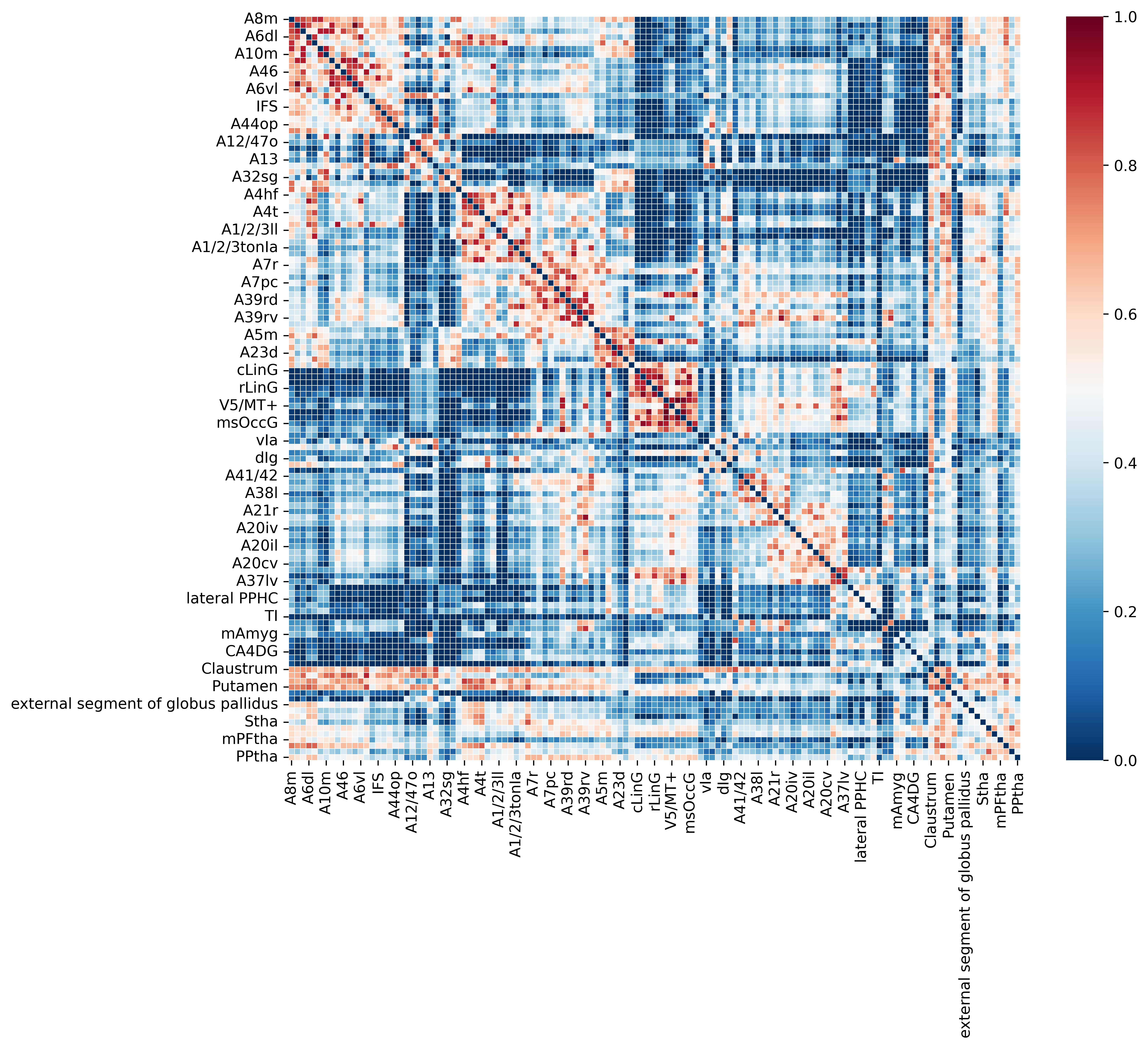
Visualization of final obtained cross-species average graph embeddings

f, ax = plt.subplots(figsize=(14, 11), dpi=300)

heatmap = sns.heatmap(
    embedding_map,
    cmap= bright_cmap,
    vmin=-0.8,
    vmax=1,
    linewidths=0.3,
    linecolor='#B0B0B0',
    cbar_kws={
        "orientation": "vertical",
        "shrink": 0.8,
        "aspect": 20,
        "label": ""
    }
)

cbar = heatmap.collections[0].colorbar
cbar.ax.tick_params(labelsize=14)

ax.set_xlabel("Regions", fontsize=24, labelpad=10, fontproperties=custom_font)
ax.set_ylabel("Regions", fontsize=24, labelpad=10, fontproperties=custom_font)

ax.set_xticklabels(ax.get_xticklabels(), fontsize=10, rotation=90, fontproperties=custom_font)
ax.set_yticklabels(ax.get_yticklabels(), fontsize=10, rotation=0, fontproperties=custom_font)

ax.tick_params(axis='both', which='both', length=5, width=1, pad=5)
plt.xticks(fontsize=14)
plt.yticks(fontsize=14)

for spine in ax.spines.values():
    spine.set_visible(True)
    spine.set_color('black')
    spine.set_linewidth(1.5)

plt.tight_layout()

plt.show()